There are 2 ways to make Index automatically in Excel for All Excel Sheets – One is by VBA code and another by Hyperlink formula.
1. Create Automatic Index Sheet of All Sheets in Excel Using VBA
VBA Code:
Sub CreateCustomIndex()
    Dim wsIndex As Worksheet
    Dim ws As Worksheet
    Dim i As Long
    Dim wsName As String

    ' Delete existing "Index" sheet if it exists
    On Error Resume Next
    Application.DisplayAlerts = False
    Set wsIndex = Worksheets("Index")
    If Not wsIndex Is Nothing Then wsIndex.Delete
    Application.DisplayAlerts = True
    On Error GoTo 0

    ' Create a new "Index" sheet at the beginning
    Set wsIndex = Worksheets.Add(Before:=Worksheets(1))
    wsIndex.Name = "Index"

    ' Initialize row counter
    i = 1

    ' Loop through all worksheets to populate the index
    For Each ws In ThisWorkbook.Worksheets
        If ws.Name <> "Index" Then
            wsName = ws.Name
            ' Place sheet name in column C
            wsIndex.Cells(i, 3).Value = wsName
            ' Create hyperlink with "Click Here" text in column D
            wsIndex.Hyperlinks.Add Anchor:=wsIndex.Cells(i, 4), _
                Address:="", SubAddress:="'" & wsName & "'!A1", _
                TextToDisplay:="Click Here"
            i = i + 1
        End If
    Next ws

    ' Autofit columns C and D for better visibility
    wsIndex.Columns("C:D").AutoFit

    MsgBox "Index sheet created successfully!", vbInformation
End Sub
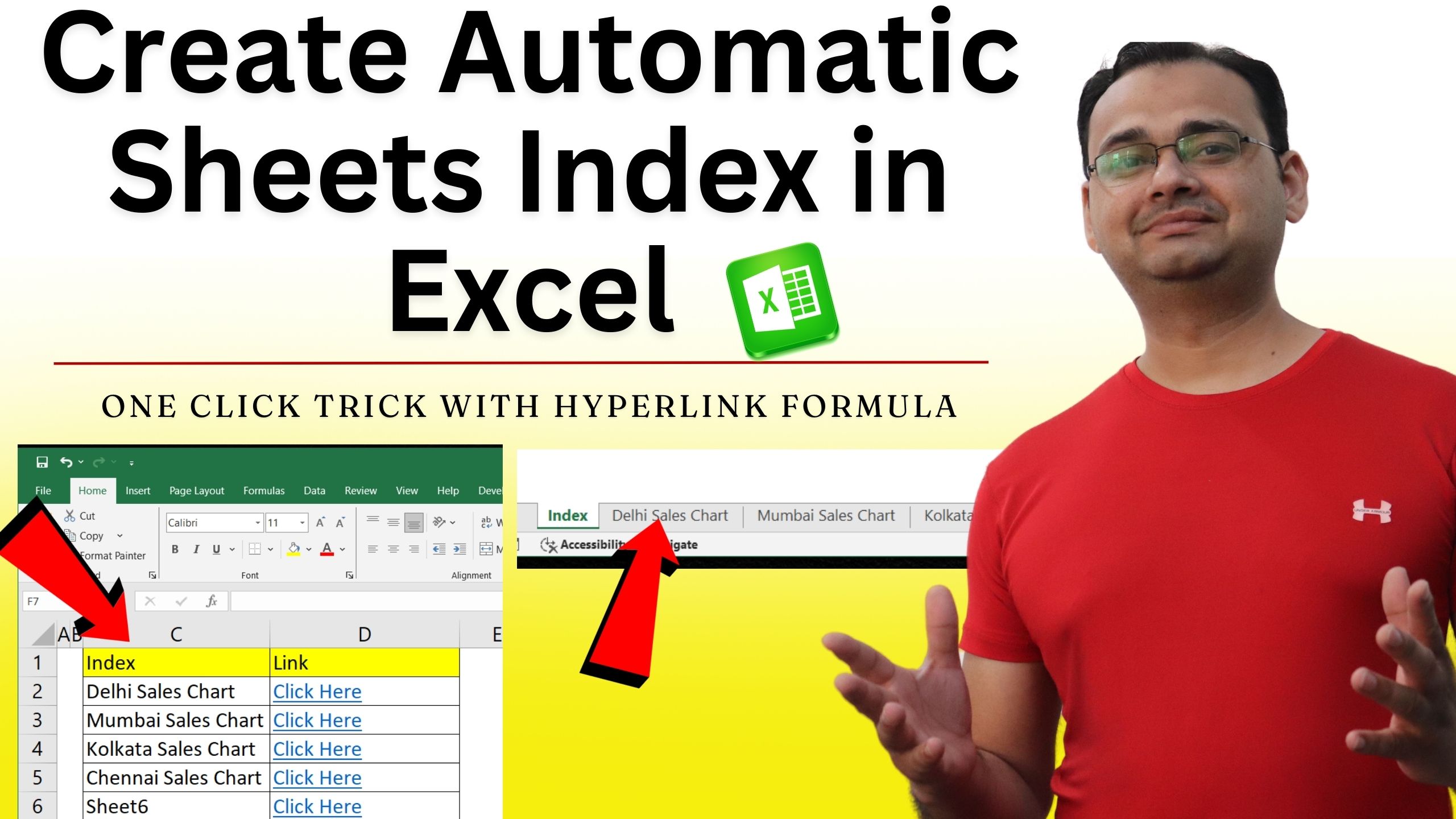
2. Create Automatic Index Sheet of All Sheets in Excel Using Hyperlink Formula
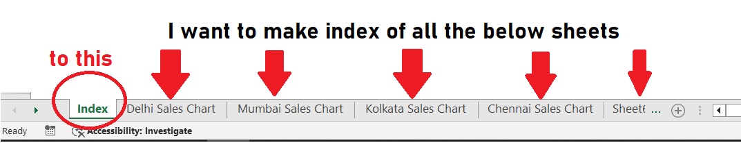
If you work with large Excel files that contain multiple sheets, navigating between them can be time-consuming. To save time, you can create an Index Sheet with clickable links to each worksheet. This way, you can jump to any sheet instantly with just one click. Here’s how you can do it using the HYPERLINK formula in Excel.
Formula to Create Hyperlinks in Excel
=HYPERLINK("#'"&C2&"'!A1","Click Here")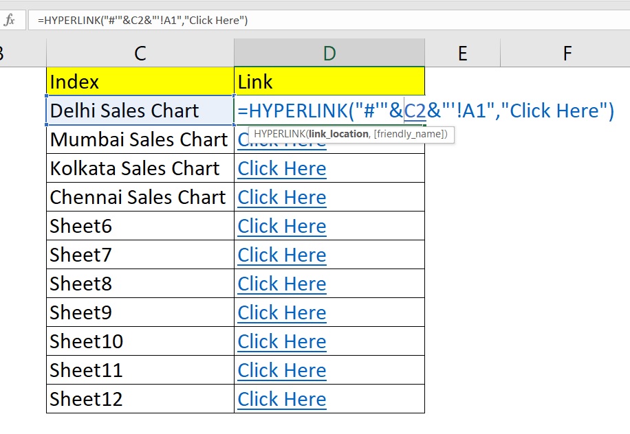
Explanation of the Formula
- =HYPERLINK(…) → Creates a clickable hyperlink inside Excel.
- “#'”&C2&”‘!A1” → This tells Excel to jump to Cell A1 of the sheet name written in Cell C2.
- “Click Here” → This is the text displayed in the cell as the clickable link.
So, if C2 contains Delhi Sales Chart, the formula will take you directly to cell A1 of that sheet when you click the link.
Benefits of Using Hyperlink Formula
- Quickly navigate between multiple sheets in a workbook.
- Makes reports look professional and easy to use.
- Reduces manual scrolling and searching for sheet tabs.
- Useful for dashboards, MIS reports, and presentations.
- You can change “Click Here” to display the sheet name instead, e.g.:
=HYPERLINK("#'"&C2&"'!A1",C2) - If you want to go to a different cell (e.g., B5), replace A1 with B5.
- This formula works even if your sheet names contain spaces, thanks to the
'(single quotes).
By using the HYPERLINK function in Excel, you can build a powerful Index Page that acts like a navigation menu for your workbook.
 Join Our WhatsApp Group


Nazim Khan (Author) 📞 +91 9536250020
[MBA in Finance]
Nazim Khan is an expert in Microsoft Excel. He teaches people how to use it better. He has been doing this for more than ten years. He is running this website (TechGuruPlus.com) and a YouTube channel called "Business Excel" since 2016. He shares useful tips from his own experiences to help others improve their Excel skills and careers.


