
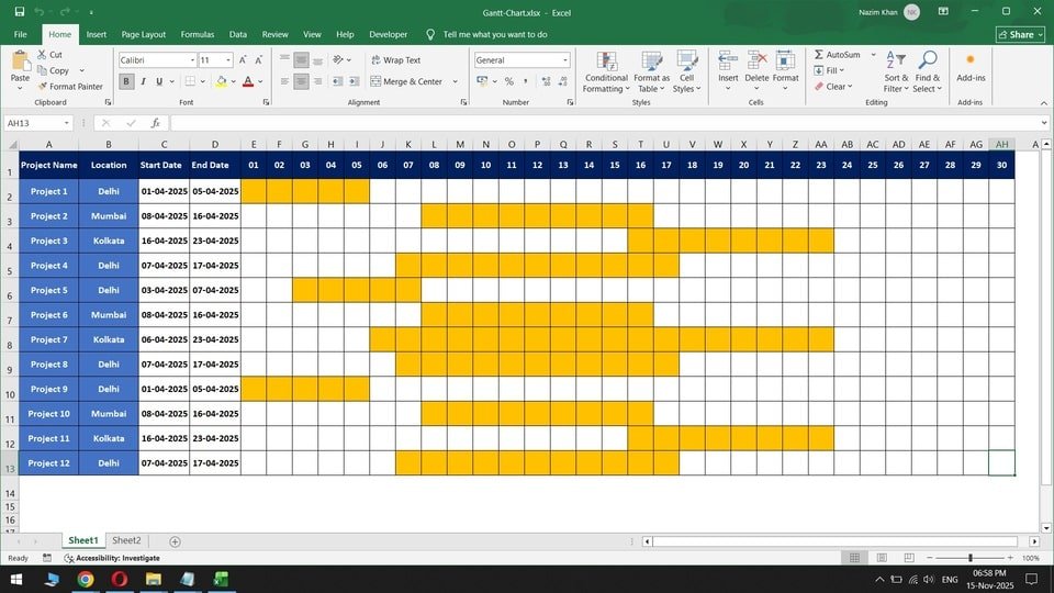
If you’re managing projects in Excel and want a visual representation of your project timelines, creating a Gantt chart with conditional formatting is a slick move. Here’s how you can do it like a pro. A Gantt chart is basically a bar chart that shows project timelines. It helps you visualize when projects start, how long they run, and when they wrap up.
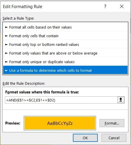
Formula for Conditional Formatting: =AND(E$1>=$C2,E$1<=$D2)
What it does:
This formula checks if the date in row 1 (like E$1) falls between the start date ($C2) and end date ($D2) of a project. If it does, the cell gets highlighted.
How it works:
E$1>=C2 checks if the date in E1 is on or after the start date.
E$1<=D2 checks if the date is on or before the end date.
AND ensures both conditions are true for highlighting.
Conditional Formatting:
- Select the range where you want the Gantt bars (like columns E to AH).
- Go to Home > Conditional Formatting > New Rule.
- Use the formula
=AND(E$1>=$C2,E$1<=$D2). - Pick a fill color (like yellow) and hit OK.
This Gantt chart lets you quickly see overlapping projects, project durations, and gaps between projects in cities like Delhi, Mumbai, or Kolkata.
Now you’ve got a dynamic Gantt chart in Excel that highlights project timelines based on start and end dates.
 Join Our WhatsApp Group


Nazim Khan (Author) 📞 +91 9536250020
[MBA in Finance]
Nazim Khan is an expert in Microsoft Excel. He teaches people how to use it better. He has been doing this for more than ten years. He is running this website (TechGuruPlus.com) and a YouTube channel called "Business Excel" since 2016. He shares useful tips from his own experiences to help others improve their Excel skills and careers.


