Pivot Table is a very important command in MS Excel. It reduces our working time and reduces the chances of error in calculation. So, first of all I want to tell you what we can do with the help of pivot table-

We will take an example to understand the pivot table in MS Excel.

Example of Pivot Table:-

We have an excel data sheet that contain Name of Company, Sale Amount and Sales Tax Amount. In this sheet the name of company are repeating as the sales made by them. Now we want to know the total amount of sales along with sales tax amount in total per company. So now we will use pivot table to get it.

Company Name	Sale Amount	Sales Tax @ 5%
Dayawati Industries	2381	119
Artemis Medicare	29800	1490
Adlife Enterprises	22857	1143
Artemis Medicare	1232	62
Adlife Enterprises	22857	1143
Advance Fertility	12381	619
Advance Fertility	12381	619
All India Medicos	2400	120
Adlife Enterprises	22857	1143
All India Medicos	4000	200
D.N. Hospital	4952	248
Adlife Enterprises	22857	1143
Artemis Medicare	25670	1284
Dayawati Industries	24762	1238
Artemis Medicare	4286	214
Artemis Medicare	1440	72
Adlife Enterprises	3526	176
Dayawati Industries	5930	297
D.N. Hospital	2560	128
Grand Total	229129	11458

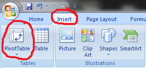
Now select the entire table of data (do not select “Grand Total” Column) then click on “insert” button and click on “Pivot Table” Button.

Create Pivot Table:-

Now a window will appear that will ask for Select a Table or Range, So enter the table range or it will take automatically as we already selected before clicking the Pivot Table Button.

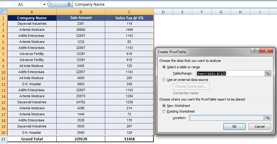
Now Click on OK button at the bottom of window.

After clicking OK Button a new excel worksheet will be open that will show the below result.

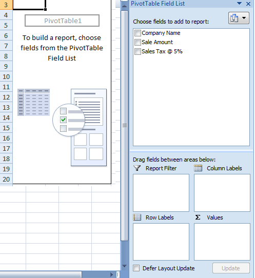
Now Click on Company, Sales Amount and Sales Tax @ 5% Check Box Button in PivotTable Field List at the right side in the excel worksheet.

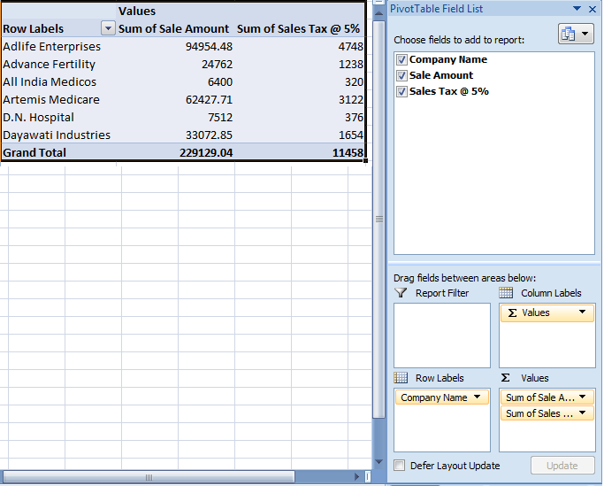
So you can see in the excel worksheet that your Pivot Table is ready and showing the result as you want. This is showing the name of company with their total sale amount along with their Sales tax amount.

Ok, Now further let me tell you one more thing that, if you change any value or name or anything in your main data sheet the result will also be changed, you just need to right click on the Pivot Table and just click on Refresh button, immediately your Pivot Table data will be change as per your data correction.

Refreshing of Pivot Table:-

Here is an image which showing where is your refresh button in pivot table.

So friends that’s it for pivot table in Microsoft Excel if you have any question or suggestion, feel free to comment in the comment box we will definitely solve your problem in the next article on our website TechGuruPlus.com