Introduction
VLOOKUP stands for ‘Vertical Lookup’. It is a formula or function which makes Excel search for a certain value in a column.
Purpose
To find information in a large spreadsheet, or looking for the same kind of information, we mostly use the VLOOKUP function. You will get to know, how to use the VLOOKUP function.
The VLOOKUP indicate, what you want to look up, where you want to find for it, the column number in the range that include the value to return, return an Approximate or Exact match.
Learning Objects
- VLOOKUP FUNCTION/FORMULA
Step by Step Process for VLOOKUP Function
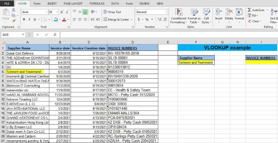
- In this example we have a list of Suppliers, invoice date, invoice creation date and the invoice number. We want to find the invoice number of supplier “Tumnem and Townmend” from this table.
Select a cell, you want to import the invoice number:

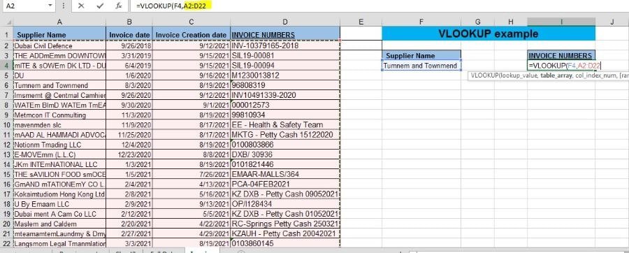
Start typing: =VLOOKUP ( “to get the data published”)

Then we select the value we want to look up, in this case it’s ‘Tumnem and Townmend’ in cell F4:

Then enter comma ‘,’ and the range, to find the lookup value and the return value. As per below case, the range is (A2:D22):

After that Enter ‘,’ and then the column number of defined range in where the return value may populate. In below case it is column 4, followed by ‘,’ and ‘0’ or ‘FALSE for an exact match with the lookup value.

=Vlookup(F4,A2:D22,4,0)
When we press enter, we get the corresponding Invoice number from the row that contains value ‘Tumnem and Townmend’ within the selected table array:

Conclusion
In this example we only have a small list of Suppliers, but imagine you have a long list of data and you wish to find certain value elsewhere in your spreadsheet. By using VLOOKUP function the user may find the unbelievable results.


