
If you want to remove blank rows, then I am going to tell you 3 ways to remove blank rows in Excel in some easy steps.
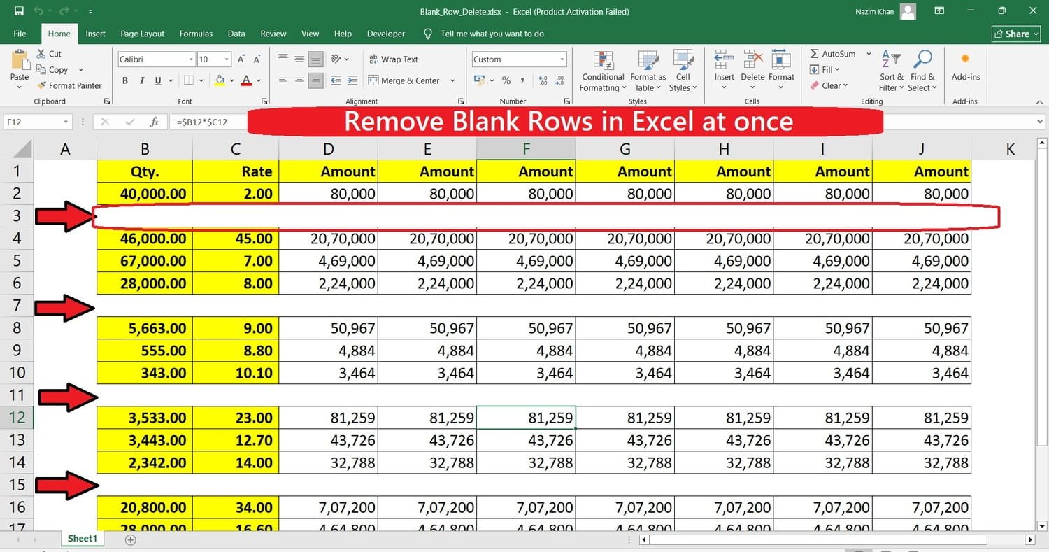
1. Using the Sort Function
First of all, insert a column at the beginning and put Serial No. in Column A. Then drag the serial numbers down to the last row of your data. Now select your complete data and apply Sort by Column B. All the blank rows will move to the bottom of your data. Select these blank rows, right-click, and delete them.
Now, to bring your data back to the original sequence, simply sort the data again by Column A (Serial No.). Once the data is back in its original order, you can delete the Serial No. column.
2. Using the Filter Function
First, select your complete data and apply Filter from the Data tab. Now open the filter dropdown and select Blanks to display only the blank rows.
After filtering the blank rows, select all the visible rows and press Alt + ; (semicolon) to select only the visible cells. Then right-click on the selected rows and choose Delete Row. Finally, remove the filter, and all the blank rows will be removed.
3. Using the Filter & Sort Function
This method is similar to the first method. First, insert a Serial No. column at the beginning and fill it with serial numbers. Then apply Filter to your data.
Go to the filter dropdown and use the Sort option to move the blank rows to the bottom. Now select the blank rows and delete them. After that, sort your data again by Column A (Serial No.) to bring the data back to its original sequence. Finally, you can delete the Serial No. column.
Video Tutorial
Join Our Telegram Group

Join Our WhatsApp Group