Excel Conditional Formatting: Color Negative Numbers Red and Positive Numbers Green (With Formula)
In Excel, Conditional Formatting allows users to visually highlight data based on specific rules. One popular use case is to color-code positive and negative numbers — for example:
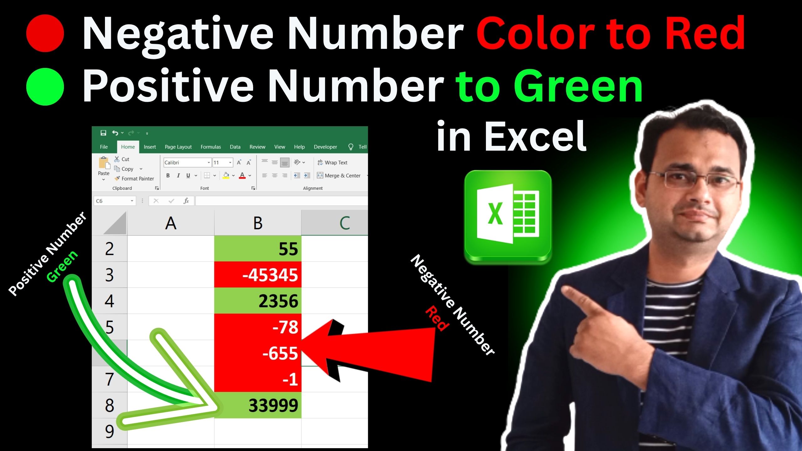
- ✅ Positive numbers → Green
- ❌ Negative numbers → Red
You can easily do this using formulas in Conditional Formatting. Let’s walk through it using your provided formulas and the example shown in the image.
Example Reference
Refer to the image :
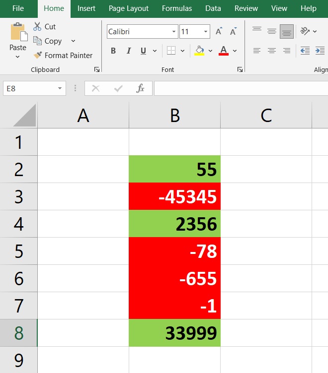
Column B (from B2 to B8) contains both positive and negative numbers. You can see that:
- Positive numbers (like
55,2356,33999) are filled green with black text. - Negative numbers (like
-45345,-78,-655,-1) are filled red with white text.
Step-by-Step Guide Using Formula-Based Rules
1. Select the Data Range
Select the range you want to apply formatting to — here, it’s B2:B8.
2. Open Conditional Formatting
- Go to the Home tab
- Click on Conditional Formatting
- Select New Rule
3. Choose “Use a formula to determine which cells to format”
Now you will enter the formulas you mentioned:
🔴 Rule for Negative Numbers (Red Background)
=$B2<=0Click Format, and choose:
- Fill color: Red
- Font color: White
🟢 Rule for Positive Numbers (Green Background)
=$B2>0Click Format, and choose:
- Fill color: Green
- Font color: Black
Notes:
- Make sure the dollar sign is in front of the column letter only (
$B2) to apply formatting correctly down each row. - These formulas evaluate the value in column B, row by row.
Now, Any updates to the numbers will instantly reflect the correct formatting.
 Join Our WhatsApp Group


Nazim Khan (Author) 📞 +91 9536250020
[MBA in Finance]
Nazim Khan is an expert in Microsoft Excel. He teaches people how to use it better. He has been doing this for more than ten years. He is running this website (TechGuruPlus.com) and a YouTube channel called "Business Excel" since 2016. He shares useful tips from his own experiences to help others improve their Excel skills and careers.


