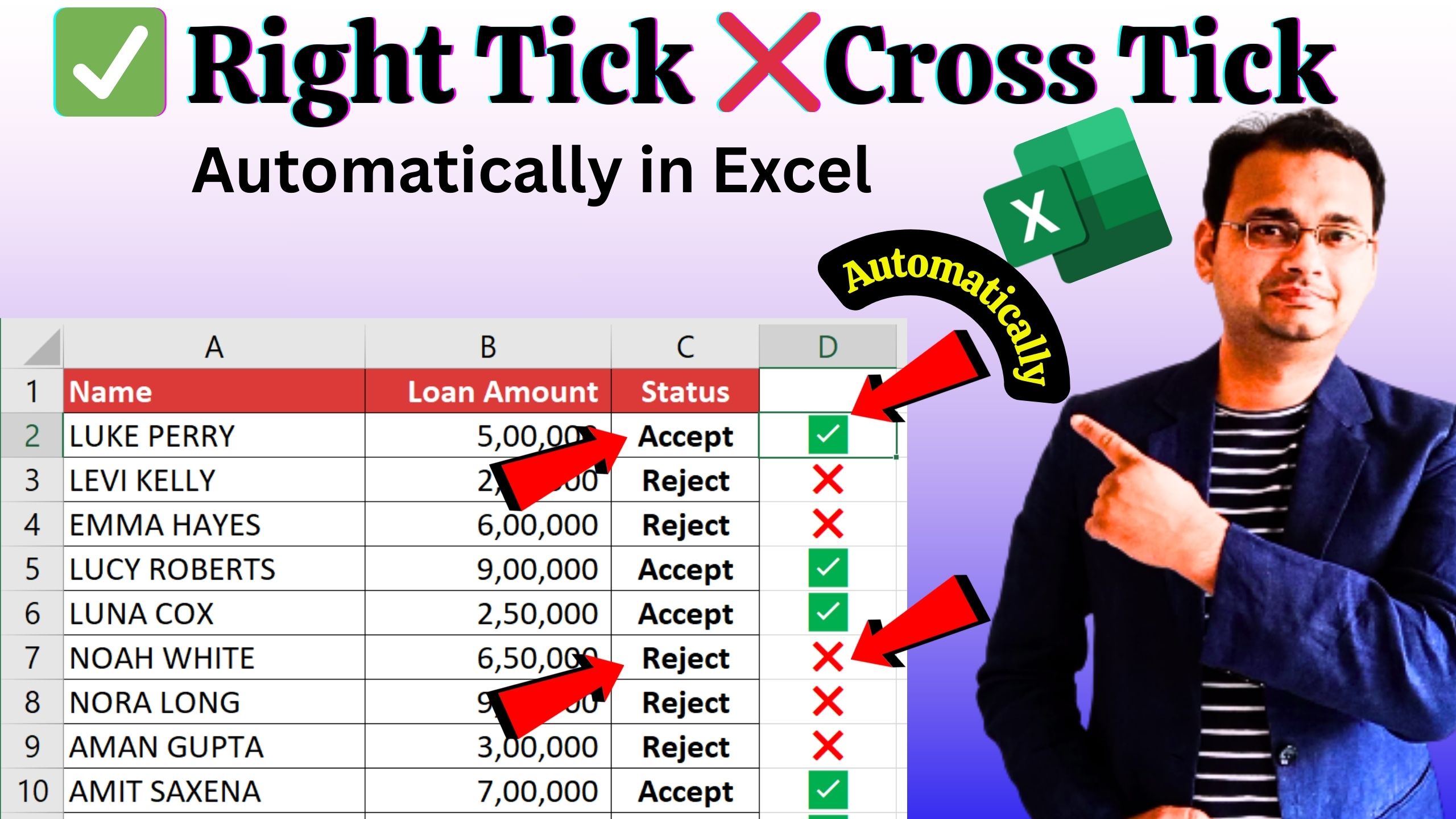
Automatic Right Tick (✅) & Cross Tick (❌) in Excel Using IF Formula
Excel is a powerful tool for data analysis and reporting, and sometimes we want to make our reports more visual and easy to understand. Instead of just writing Accept or Reject, you can use Right Tick (✅) for Accepted and Cross Tick (❌) for Rejected records automatically. This can be done easily with the IF formula in Excel.
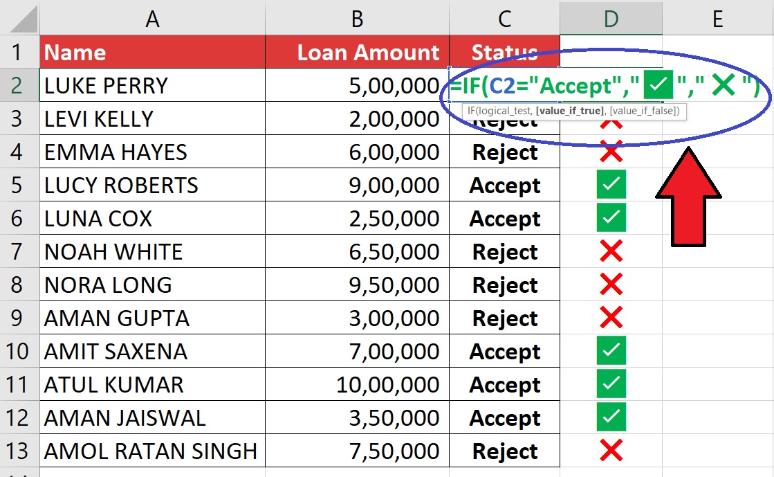
Formula to Insert Tick & Cross
=IF(C2="Accept","✅","❌")Explanation of the Formula
- =IF(…) → This checks a condition and returns different results based on TRUE or FALSE.
- C2=”Accept” → The condition. If the value in cell C2 is “Accept”, then Excel will return a Right Tick (✅).
- “✅” → Value if the condition is TRUE (Accept).
- “❌” → Value if the condition is FALSE (Reject).
- You can replace “✅” and “❌” with any other symbol, emoji, or even text (like “Yes” / “No”).
- If you want to change the condition (e.g., check for “Yes” instead of “Accept”), just update the formula:
=IF(C2="Yes","✅","❌") - Combine with Conditional Formatting to highlight cells with color for even better visualization.
Join Our Telegram Group

Join Our WhatsApp Group